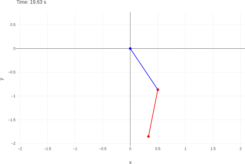
In this article, I explain to Fidello from Foci's Discord server some prerequisite knowledge he needs to effectively derive the equations of motion for a double rigid pendulum and then cover more advanced topics for him. In theory, the derivation of the equations of motion for a double rigid pendulum can be done with Newtonian mechanics with $\textbf{F}=m\mathbf{a}$, but given our second pendulum is in a moving reference frame and Newtonian mechanics does not easily adapt to alternative coordinate systems, like polar coordinates, Lagrangian mechanics makes the equations of motion easier to derive. Lagrangian mechanics also leads nicely into Hamiltonian mechanics and the path integral formulation of quantum mechanics. Figure shows a frame from the double pendulum animation this page does by default.

Prerequisite mathematics

There are several pieces of prerequisite mathematics I need to cover in order for this article to make sense for you.

Maclaurin and Taylor series

If we have a function $f(x)$, it is usually possible to write an infinite sum (or series) that equals $f(x)$ using $f(x)$'s derivatives.Namely:

Where we are using $\dfrac{d^n f}{dx^n}\Big|_{x=a}$ to denote the $n$th derivative of $f(x)$ evaluated at $x=a$ and $n!$ denotes the factorial of $n$. If you are unfamiliar, well $n!=n\times (n-1) \times (n-2) \times(n-3) \times ... \times 1$. For instance, $5!=5\times 4 \times 3 \times 2 \times 1=120$. As for $a$ it is an arbitrary number we get to choose. Equation (1) is known as the Taylor series of $f(x)$.

If $a=0$, then we get the Maclaurin series:

Why do these equations hold? Well, try taking the $n$th derivative of Equations (1) and (3) and substituting $x=a$ and $x=0$, respectively. You'll find that you get $\dfrac{d^n f}{dx^n}\Big|_{x=a}$ and $\dfrac{d^n f}{dx^n}\Big|_{x=0}$, respectively. Consequently, our series matches our original function in its $n$th derivative for $n\in \mathbb{Z}^{+}$. Likewise, if you substitute in $x=a$ and $x=0$ into the Taylor and Maclaurin series, respectively, you should get $f(a)$ and $f(0)$, respectively. So we see that this is like a polynomial of infinite order that matches our original function for its value and derivatives value at one point. It turns out that this means it contains enough information to match our original function at other points, too.

There are exceptions where Taylor series do not accurately compute the function they pertain to. For instance, points where the function is undefined can mess things up. As an example, $\ln{(x+1)}$'s Maclaurin series will only approximate $f(x)$ well for $-1 < x < 1$ as at $x=-1$ the function is undefined. Beyond these points it will fail to converge (meaning it will not equal some finite number as terms for higher $n$ will not get rapidly smaller as $n$ gets bigger).

Now, I know this probably seems pretty abstract to you right now. But let us try to figure out the Maclaurin series for some example functions for which the $n$th derivative is fairly easy to calculate. Say, for instance, we calculate the Maclaurin series for $e^x$. Why $e^x$? Because the $n$th derivative of $e^x$ is just $e^x$, and evaluating this at $x=0$ yields 1. Hence:

is the Maclaurin series of $e^x$. Okay, let us try our hand at another function's Maclaurin series. How about $\cos{x}$? We know the first derivative of $\cos{x}$ is $-\sin{x}$. Hence the second derivative is $-\cos{x}$. The third derivative would be $\sin{x}$. Fourth derivative would be $\cos{x}$. Fifth derivative would be $-\sin{x}$ and sixth derivative would be $-\cos{x}$. Well, I have noticed a pattern here! Seems to me like $(-1)^{\lfloor\frac{n+1}{2}\rfloor}$ (where $\lfloor ... \rfloor$ rounds down decimals, e.g. it would take 3.6 and return 3) will recreate the sign of this function. If $n$ is even, the trigonometric function will be $\cos{x}$ and if it is odd it will be $\sin{x}$. Evaluating these functions at $x=0$, we see that if $n$ is even we will get $1$ from the trigonometric function and 0 if $n$ is odd. Hence:

So our sum will essentially just be over even numbers. One way we can denote a sum over even numbers is by replacing $n$ with $2n$ and summing over all numbers. As $2$ times any integer is always an even number. In this event, our $(-1)^{\lfloor\frac{n+1}{2}\rfloor}$ becomes:

We arrived at Equation (6) simply because $n$ is an integer so adding a half to it should make no difference when we are rounding down. Consequently, our Maclaurin series becomes:

So here is some homework for you: try constructing the Maclaurin series for $\sin{x}$. You should arrive at:

As another example, we will find the Maclaurin series for $\ln{(x+1)}$ so we can see why it only converges well for $|x| < -1$ where $|x|$ is the absolute value of $x$. The first derivative is $\dfrac{1}{x+1}$. Second derivative is $-\dfrac{1}{(x+1)^2}$. Third derivative is $\dfrac{2}{(x+1)^3}$. Fourth derivative is $-\dfrac{6}{(x+1)^4}$. So it seems to me that the pattern is that the numerator is $(-1)^{n-1} (n-1)!$ and the denominator is $(x+1)^n$. Hence:

And: Hence our Maclaurin series is: If $|x|>1$, we would expect the power of $x$ in our numerator to potentially grow faster than $n$ and hence our terms could become progressively larger as $n\rightarrow \infty$. As for if $x=\pm 1$, well our numerator would be smaller than our denominator, but our denominator would grow rather slowly, which means we would have to calculate a lot of terms to figure out what value it ends up equalling, assuming it does converge. If $x=1$, we get: Which is actually true. As this sum does, indeed, equal $\ln{2}$. But because the denominator grows very slowly, we would need a lot of terms in the series in order to get a good approximation for what it equals. If $x=-1$, then we get: This sum does not converge, hence it actually equals $\infty$. Hence why $|x| < 1$ is a requirement for this Maclaurin series to converge, or at least converge at a reasonable pace, although it does also converge, albeit slowly, for $x=1$.

Maclaurin and Taylor series have broad applications in physics. One application they have is in helping us connect more general and robust laws of physics to older approximations. For more on this, see the section on the classical limit of special relativity's kinetic energy.

Complex numbers

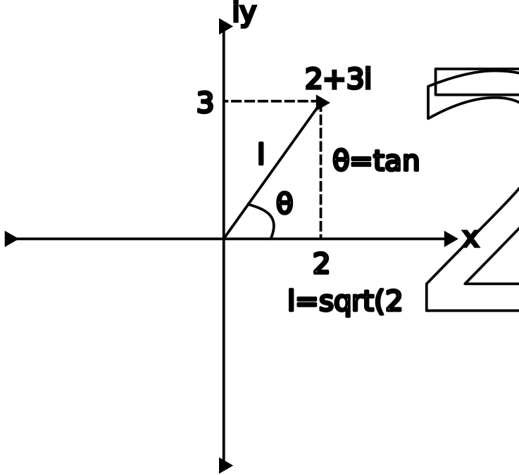
Complex numbers are numbers that involve both a real and an imaginary part. That is, they are of the form $a+bi$ where $a$ and $b$ are both real numbers and $i$ is the imaginary number. $a$ is called the real part of the number and $b$ is called the imaginary part of the number. Importantly, $a$ and $b$ can be zero, consequently all real numbers are technically complex numbers. We can display complex numbers in the complex plane (also known as the Argand plane) as vectors. Specifically, the $y$ component of this vector is the imaginary part of our number and the $x$ component is the real part of the number.

Figure shows the number $2+3i$ displayed in the complex plane. The length of the vector, $l$, can be calculated using the Pythagorean theorem as $l=\sqrt{2^2+3^2}=\sqrt{13}$. $l$ can also be called the modulus of our complex number. As for $\theta$, the angle from the positive $x$-axis measure counterclockwise it can be found using the definition of the tangent function as $\theta =\tan^{-1}{\dfrac{3}{2}}$. Note also that $3=l\sin{\theta}$ and $2=l\cos{\theta}$ by the definition of these trigonometric functions.

Interestingly, these two qualities, the length of the complex number's vector and its angle, measured counterclockwise from the positive $x$-axis, can be used to uniquely define it. To see how, I must first share with you an interesting quality of the exponential function. Namely, that:

Why is this the case? Replacing $x$ with $iz$ in Equation (5) yields: You may be thinking, so what? Well, powers of $i$ have interesting properties. Namely, $i^0=1$, $i^1=i$, $i^2=-1$, $i^3=-i$ and $i^4=1$. Generally, $i^{4n}$ (where $n$ is an integer) is equal to $1$, $i^{4n+1}$ is $i$, $i^{4n+2}$ is $-1$ and $i^{4n+3}$ is $-i$. Focusing on even powers, we find that $i^{2n}=(-1)^n$ (where makes sense as $i^2=-1$ and $i^{2n}=(i^2)^n$). Whereas odd powers yields $i^{2n+1}=(-1)^n i$. Consequently: The first of these sums we can recognize as $\cos{z}$ whereas the second is $\sin{z}$. Hence: An interesting thing to note that $e^{iz}$ is that its modulus is one. How do I know this? Well, the modulus is defined as just the length of the complex number's vector in the complex plane, right? So for $e^{iz}$ that would be: Here I used the trigonometric identity: Where $\mathbb{R}$ is the set of real numbers. Okay, so getting back to how $l$ and $\theta$ can uniquely define a complex number. Well, interestingly you can write any complex number in the form $le^{i\theta}$. Why? Well, recall that $e^{i\theta}$ is just $\cos{\theta}+i\sin{\theta}$. Looking at Figure we can clearly see that the $x$ component of our vector is just $l\cos{\theta}$, right? And we can also see that the $y$ component is just $l\sin{\theta}$ and if we expand our $le^{i\theta}$ we get: Hence $le^{i\theta} = x+iy$. For instance, for the complex number $2+3i$ we can rewrite it as:

Complex analysis

I have definitely not covered everything within the field of complex numbers. There's a field of maths known as complex analysis where we combine calculus and complex numbers. In it, we learn, among other things, how to integrate along curves (or contours) in the complex plane and that there is an extension of Taylor series to the complex plane called the Laurent series. In it, we write:

where: This is a contour integral over a curve $C$ that includes the point $z=z_0$. $z_0$ is analogous to the $a$ in our Taylor series as it is arbitrary. There's a formula called Cauchy's differentiation formula that says that: Where $f^{(n)}(z_0)$ is the $n$th derivative of $f(z)$ evaluated at $z=z_0$. Which helps us see how the Laurent series is connected to the Taylor series as for non-negative $n$, $a_n = \dfrac{f^{(n)}(z_0)}{n!}$. As for negative $n$, $a_n=0$ if $f(z)$ is defined everywhere in the complex plane. Why do I mention this? Well, I personally consider complex analysis one of the most beautiful fields of mathematics and I thought I would mention it in case you are ever in a position to take a complex analysis class while at university.

Partial derivatives

Partial derivatives are just a straightforward extension of derivatives as you understand them already. The key difference is that they are derivatives of multivariable functions instead of single-variable functions. Further, when you differentiate with respect to one variable, all other variables are kept constant. If you would like to build a graphical image of what the partial derivative is, well recall that the derivative of a single-variable function is just the gradient of that function. Consequently, it is also the gradient of the tangent line to that function. The partial derivative is similar to that. As when we have a function with more than a single independent variable, we have the freedom to choose which variable or variables we wish to determine our function's gradient with respect to.

If you want to visualize this, imagine a surface defined by $z=f(x,y)$ for example. Because a tangent line is two dimensional and we're in three dimensional space, there can be more than one tangent line to a given point. As when constructing the tangent line, we must answer a question: in which direction do we want our line to be tangential to our surface? It could be tangential in the $x$ direction or the $y$ direction, or even in any arbitrary direction in the $xy$ plane. If we want the tangent line in the $x$ direction, we will need the partial derivative with respect to $x$ to get its gradient, whereas if we want the tangent line in the $y$ direction, we will need the partial derivative with respect to $y$ to get its gradient. More generally, for an arbitrary direction in the $xy$ plane we would use the directional derivative as it is called.

Say $f$ is a function of two variables — $x$ and $y$. Then its partial derivative with respect to $x$ is formally defined as:

This is analogous to the first principles definition of the derivative you would have learned for standard derivatives. Namely, if we are differentiating $f(x)$:

The only difference is that now we also have a variable $y$ that our function $f(x,y)$ depends on, but is kept constant when differentiating with respect to $x$. Say $f(x,y)=2x^2y$. Then $\dfrac{\partial f}{\partial x}$ would be: Did you notice that $2y$ is a common factor of both terms in our numerator? Let us take it out of our limit altogether, as it is effectively a constant (it does not depend on $h$, after all).

Using the binomial theorem, we know that

Hence:

Okay, so that is the long way of finding out partial derivatives. Fortunately, there is also a faster way. Which is that we apply normal differentiation rules, but any variable we are not differentiating with respect to is treated like it is a constant. So for $f(x,y)=2x^2y$ we would treat the $2y$ as just a constant number and only differentiate the $x^2$. Applying the power rule, we see that $\dfrac{d}{dx}x^2 = 2x$ and hence:

Heat equation

One of the simplest partial differential equations is the heat equation. In its simplest form it is:

Where $u(x,t)$ is a function describing the temperature of the one-dimensional object (only one dimensional as the above heat equation only has a single spatial dimension, if we want more spatial dimensions we'll have to add second partial derivatives with respect to those other dimensions, too) we're modelling and $\alpha$ is some constant. I know this equation may look confusing at first glance, but it is actually saying something rather intuitive to you.

Do you remember from your maths class that the second derivative of a function is its concavity? So if the second derivative is negative, that means our function is concave down — it is leading to some sort of maximum. Whereas if it is positive, the function is concave up, which means it is going up from some minimum. We have the second derivative with respect to space on the right-hand side of Equation (18), so it essentially returns positive if we have a localized colder area and neighbouring hotter points. Whereas it returns negative if we have a really hot point surrounded by cooler points. The left-hand side of Equation (18), however, represents the rate of change of our function in time.

Equation (18) therefore essentially says that if we are in a region where there is a really cold point surrounded by hotter points, the temperature will increase in the short-term for that colder point. Whereas the equation says that the temperature will decrease in a hotter region surrounded by colder points. If you've ever brought something hot out of the oven, or put something of room temperature into the fridge or freezer, this should make intuitive sense to you.

Lagrangian mechanics

Lagrangian mechanics is one of three major formulations of classical mechanics with the others being Newtonian mechanics and Hamiltonian mechanics. Classical mechanics as a whole is a branch of physics most applicable to the situations that humans most often encounter, as it does not account for quantum randomness (hence cannot be applied to very small scales), nor does it account for relativistic effects (which are most relevant when dealing with strong gravitational fields or velocities close to the speed of light). In Lagrangian mechanics, we define a quantity known as the Lagrangian of our physical system:

Where $T$ is kinetic energy and $V$ is potential energy of our entire physical system. It is important to note that only conservative forces contribute to $V$. Lagrangian mechanics can account for non-conservative (i.e. dissipative) forces, too, but we will get to how one handles them later.

The distinction between conservative and non-conservative forces is whether they change the net energy of your system. For instance, gravity does not because any increase in kinetic energy it causes is balanced by a corresponding reduction in potential energy. Likewise, any loss of kinetic energy caused by gravity is balanced by an increase in potential energy. Consequently, it is a conservative force. Air resistance, however, is a non-conservative force because the losses it causes in kinetic energy are not balanced by increases in potential energy.

Euler-Lagrange equations

When there are no non-conservative forces, the equations of motion can be derived by first determining our system's Lagrangian and then applying a set of partial differential equations known as the Euler-Lagrange equations to this Lagrangian. The Euler-Lagrange equations are:

$q_i$ are the $n$ degrees of freedom (or generalized coordinates) of our problem and $\dot{q}_i$ are their time derivatives (or the generalized velocities). The $\dfrac{d}{dt}$ is not a partial derivative and this is purposeful, as when we differentiate $\dfrac{\partial L}{\partial \dot{q}_i}$ with respect to $t$, we treat $q_i$ and $\dot{q}_i$ as functions of $t$ and wherever they appear in $\dfrac{\partial L}{\partial \dot{q}_i}$ we differentiate them against $t$.

Next, I should explain what "degrees of freedom" are. They are essentially our variables of interest. For simpler problems, the degrees of freedom in our problem are often the spatial dimensions of our problem. For instance, if we were to study an object in free fall and we were to try to simplify our problem as much as possible and not consider any movement in the horizontal directions then $n$ could be 1 and $q_1$ would just be the height of the object above ground level.

Likewise, when we study the simple pendulum — which is a problem in which we have an idealized rigid pendulum whose rod has zero mass, zero friction and for which there is absolutely no air resistance — typically we only consider a single degree of freedom, which is the angle our pendulum's rod makes with either the negative $y$ axis or the positive $x$ axis, depending on the preferences of whoever is setting up the problem.

Derivation of Equations (20)

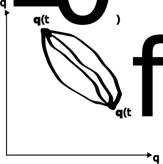
The derivation of Equations (20) requires knowledge of a field of mathematics known as the calculus of variations as well as a physics principle known as the stationary action principle. I will provide my own derivation here; although, I would suggest checking out Veritasium's video on this topic (https://www.youtube.com/watch?v=Q10_srZ-pbs) as it provides a more accessible introduction to this topic.

There is a quantity known as the action — which is denoted as $S$ — that is defined as:

One interesting property of the action is that nature consistently sets it to its stationary point, and this is regardless of context. Regardless of whether we are examining the motion of planets with Newton's second law, or studying the behaviour of black holes with general relativity, or checking out the behaviour of subatomic particles, there is always an action that is at its stationary point. Traditionally, this stationary point is typically thought of as a minimum (hence why this is also known as the principle of least action), but strictly speaking it is not always a minimum.

Of all the paths that an object could explore, the one that it actually explores is the one that sets the action to its stationary point. Figure provides some example paths that we examine when applying the principle of stationary action. In the terminology of the calculus of variations, we can express the fact the action is at its stationary point as:

This is analogous to saying, in regular calculus, that our function's first derivative is zero. Which, as you may remember from your maths classes, is an equation we can solve to find the stationary point(s) of our function.

Say we add functions $\delta q_i$ to $q_i$, thereby adjusting the path our object takes. Crucially, however, the end times and end points of our path will be unchanged. The new, adjusted action we will denote by $S'$ and it is:

Next, we will apply integration by parts to the $\dfrac{\partial L}{\partial \dot{q}_i}\delta \dot{q}_i$ term:

At the end times of our path, $\delta q_i$ should be zero, as the endpoints are fixed. Hence the term $\left[\dfrac{\partial L}{\partial \dot{q}_i}\delta q_i\right]_{t_0}^{t_f}$ should evaluate to zero. Our expression then simplifies to: The first of these terms is present in $S$, too. Hence: We can denote this first-order approximation to how much $S$ changes as $\delta S$. Hence: Hence $\delta S$ will equal zero irrespective of $\delta q_i$ if and only if Equations (20) hold. Hence from setting $\delta S=0$ we get the Euler-Lagrange equations.

Terminology

In Equation (20):

is known as the canonical (or generalized) momentum. It becomes especially relevant later when we cover Hamiltonian mechanics.

Non-conservative forces

I guess next I should explain how we account for non-conservative forces. Essentially we replace the $0$ in Equations (20) with the generalized force $Q_i$. It is defined as:

Where $\textbf{F}_j$ represents the vector of the $j$th non-conservative force we wish to account for in our equations of motion. As you can see by the summation bounds, we have $m$ non-conservative forces we wish to account for. $\textbf{r}_j$ is the position vector for force $j$. $\textbf{F}_j\cdot\dfrac{\partial \textbf{r}_j}{\partial q_i}$ denotes the dot product between $\textbf{F}_j$ and $\dfrac{\partial \textbf{r}_j}{\partial q_i}$. Alternatively, to calculate $Q_i$ we can use velocities instead of positions: $\dot{\textbf{r}}_j$ is the time derivative of the position vector (that is, the velocity vector) for force $j$. Hence the more generalized form of Equations (20) is: The velocity-based definition of $Q_i$ can also be used, which yields:

Example: single pendulum

So to punctuate how one applies Equations (20) and (27), I thought I would give you a nice, simple example: the single pendulum.

Without air resistance

To apply Equations (20), we will treat it as a simple pendulum with no friction, a massless rod and no air resistance. The pendulum will consist of a rod with a bob at one end and freely rotating around a central point. We will define this central point as being the origin in Cartesian coordinates. Say the rod is of fixed length $l$ metres. The pendulum bob will be of mass $m$ kilograms. As you can see in Figure , we have defined $\theta$ as the angle between the rod and the positive $x$-axis going counter-clockwise. Hence the $x$ and $y$ coordinates of the pendulum bobs are:

Hence: As for velocity squared, it is defined as: Hence $v=l\dot{\theta}$. The kinetic energy is: As for potential energy, given this bob is moving solely under the force of gravity: Hence: $\dfrac{\partial L}{\partial \dot{\theta}}$ is hence: And its time derivative is: As for the $\dfrac{\partial L}{\partial \theta}$ term it is: So Equations (20) becomes: Dividing by $ml^2$ and taking the second term to the right-hand side yields: Equation (29) has, as its highest order derivative, a second-order derivative. It also only involves ordinary derivatives (not partial derivatives). Hence it is a second-order ordinary differential equation (ODE). Second-order ODEs are typically obtained in both Newtonian and Lagrangian mechanics. The number of second-order ODEs obtained for a given system depends on the number of degrees of freedom of the system.

Technically speaking it is possible to analytically solve Equation (29), but it requires the use of non-standard functions called elliptic integrals. If you would like to check out numerical solutions to this equation, see this page.

With air resistance

For the sake of simplicity, we will only consider the air resistance experienced by the pendulum bob itself, not by the rod. The air resistance force vector for the pendulum bob would be:

Where $\textbf{v}$ is the velocity vector of the bob. It is equal to $(\dot{x}, \dot{y})$. Hence: To find the generalized force term, we need to find $\dfrac{\partial \textbf{r}}{\partial \theta}$: Hence: Hence Equations (27) become: Dividing by $ml^2$ yields: Subtracting $\dfrac{g}{l}\cos{\theta}$ from both sides yields: This equation cannot be analytically solved, so numerical solutions are necessary. I numerically solve an even more complex version of the single pendulum equation here.

If you would like to see my derivation of the double rigid pendulum equations, it is here.

Hamiltonian mechanics

In Hamiltonian mechanics, we define the Hamiltonian as:

Which is the total energy of our system. I should say that this is usually the form of the Hamiltonian, more generally it is defined as: Equation (31) is called the Legendre transformation of the Lagrangian. So when are Equations (30) and (31) not equivalent? The answer is when our potential energy depends, at least in part, on the generalized velocities. Another difference from Lagrangian mechanics is that we define $H$ in terms of $p_i$ and $q_i$ instead of $q_i$ and $\dot{q}_i$.

So what is the Legendre transformation? It takes a function, say $f(x)$, and it uses its tangent lines and their $y$ intercepts to create a new function, $g(p)$ that incorporates all the information that $f(x)$ contained. Here is a great video that explains the Legendre transformation and its derivation.

The equations of motion with no non-conservative forces are:

We can derive these equations of motion by considering an infinitesimal change to our path and its effect on $H$, which we will denote as $dH$: To go from Equations (34) to (35), we used the product rule of differentiation, in case you were wondering. Next we use the definition of canonical momentum: Next we can use Equations (20) to simplify our $\dfrac{\partial L}{\partial q_i}$ term. As remember this, according to Equations (20) is equal to $\dfrac{d}{dt}\dfrac{\partial L}{\partial \dot{q}_i}$ which can also be written as $\dot{p}_i$: Assuming our Hamiltonian does not explicitly depend on $t$, we can also write $dH$ as: As this is just the change in $H$ caused directly by the change in $q_i$ plus the change in $H$ that is directly caused by the change in $p_i$. Equating like terms in the right-hand sides of Equations (36) and (37) yields: Which are Equations (32) and (33), which are known as Hamilton's equations. I should mention this is not the only way to derive Hamilton's equations; it is also possible to derive them directly from the stationary action principle, for instance.

To account for non-conservative forces, we merely add the corresponding generalized force terms to the right-hand side of Equation (32). In other words:

This creates a new kind of space that we can visualize our solution on that has dimensions $q_i$ and $p_i$. This type of space is known as phase space.

Example: simple pendulum

The Hamiltonian for the simple pendulum is:

We can use Equation (30) to determine our Hamiltonian here because our potential energy, $V$, is independent of the generalized velocities. Problem is, however, that this is written in terms of $q_i$ and $\dot{q}_i$ not $q_i$ and $p_i$. First we need to determine what our canonical momentum is. Equations (24) yields: Rewriting Equation (41) with $\dot{\theta}$ as its subject: Substituting Equation (45) into Equation (40) yields: Cancelling out common factors in the numerator and denominator of the kinetic energy term yields: Hence the equations of motion are: As we can see, Hamiltonian mechanics yields a series of first-order ordinary differential equations (ODEs) instead of second-order ODEs. Which is important because Lagrangian mechanics and Newtonian mechanics both yield second-order ODE systems. That being said, if you rewrite Equation (45) to make $p_{\theta}$ its subject and substitute it into Equation (44) and rearrange it to make $\ddot{\theta}$ the subject, you will obtain Equation (29).

Poisson brackets

Poisson brackets provide us an elegant and powerful way to rewrite Hamilton's equations. If we have $n$ degrees of freedom and two functions $f$ and $g$ that depend on $p_i$ and $q_i$:^[1]

Poisson brackets also have several interesting properties, such as antisymmetry:

Consequently: Further, assuming each of the coordinates of the phase space are independent, it follows that: Above we used $\delta_{ik}$ to denote the Kronecker delta function. It is equal to one if its arguments are equal and zero otherwise. The quality of two functions, say $f$ and $g$, having a Poisson bracket that equals zero is phrased as $f$ and $g$ commuting under the Poisson bracket.

If a function $f(q_i, p_i)$ is not explicitly dependent on $t$ and only depends on $t$ indirectly through $q_i$ and $p_i$, then, via the chain rule:

We can use Hamilton's equations to replace $\dfrac{dq_i}{dt}$ and $\dfrac{dp_i}{dt}$: Interestingly, the right-hand side is equal to the Poisson bracket of $f$ with $H$, in other words: Hence commuting with the Hamiltonian under the Poisson bracket is a sufficient condition for a quantity that does not explicitly depend on time to have a zero time derivative. A zero time derivative means the quantity is static over time which means it is conserved.

This quality makes it unsurprising that Hamilton's equations can be rewritten as:

Noether's theorem

Noether's theorem essentially states that for every continuous symmetry in the Lagrangian, there is a corresponding conservation law. For instance, time translation symmetry of the Lagrangian yields the conservation of energy. To show this, we will assume our Lagrangian does not explicitly depend on $t$. That is, $t$ itself does not appear directly in our Lagrangian. The only time dependence $L$ has on $t$ is through the dependence of $q_i$ and $\dot{q}_i$ on time. If the Lagrangian did explicitly depend on time, we would expect it not to have time translation symmetry. Say we increase time according to the transformation: $t\rightarrow t+dt$ where $dt$ is an infinitesimal change in $t$.

Subtracting $L(q_i(t), \dot{q}_i(t))$ from both sides of Equation (58) yields: We will call the left-hand side of Equation (59) $dL$, hence Equation (59) becomes: Rearranging Equations (20) yields that: If you are wondering what about if we have non-conservative forces? Would that not mean Equations (61) would not hold as there would be a missing generalized force term? Yes and in that event the Lagrangian would indeed change in time and conservation of energy would not hold, as our system would be losing energy to those non-conservative forces.

Substituting Equations (61) into Equation (60) yields:

Substituting Equations (24) into Equation (62) yields: We can rewrite the bracketed expression on the right-hand side of Equation (63) using the product rule of differentiation as: If $L$ does not change in time, $\Delta L=0$, and hence: Dividing both sides of Equations (64) by $dt$ yields: $L$ does not change, so $\dfrac{dL}{dt}=0$, too. Hence: We could now use Equation (31) to simplify Equation (65), but I would like to use this as an opportunity to show you how Equations (30) and (31) are usually equivalent. Interestingly, $\displaystyle\sum_{i=1}^n p_i \dot{q}_i=2T$, that is it is twice the kinetic energy of our system. We can establish this identity using Euler's theorem for homogeneous functions.

Say we have a homogeneous function $f$ of degree $m$ of the form:

where $a_{i,j,k,...,}$ are coefficients that do not depend on our variables. In other words, $f$ is a polynomial function of $x_i$ ($i\in\{1, 2, 3, ..., n\}$) with a maximum total power of $m$. Then Euler's theorem states that:^[2] Kinetic energy is a homogeneous function, in terms of $\dot{q}_i$, of second order, specifically it can be written as: Here also $a_{ij}$ refers to coefficients that do not depend on $\dot{q}_i$. Hence: If we assume that potential energy is independent of $\dot{q}_i$, then: Plugging Equations (69) into Equations (68) gives: Substituting Equations (24) into Equations (70) we get:

Hence if we substitute Equation (19) into Equation (65), we obtain:

Hence substituting Equation (30) into Equation (72) yields: So we see that Equations (30) and (31) are equivalent if and only if potential energy is independent of generalized velocity. We also obtain that the Hamiltonian — which is the total energy of the system if potential energy is independent of generalized velocity — does not change when the Lagrangian is time symmetric, hence it is conserved.

I should also mention that the Hamiltonian formulation of Noether's theorem uses Equation (54). As if a quantity that does not explictly depend on time commutes with the Hamiltonian under the Poisson bracket, this means it does not change over time and hence is conserved.

Hamilton-Jacobi equation

There is a final formulation of classical mechanics that I should probably cover. It is based around the so called Hamilton-Jacobi equation which is of the form:

Where $S$ is the action, which is also called Hamilton's principal function. In this approach, we essentially write our Hamiltonian in terms of $p_i$ and $q_i$ and then replace the $p_i$ with $\dfrac{\partial S}{\partial q_i}$. If our Hamiltonian does not explicitly depend on time, which is usually the case, we then use a separation of variables of the form: Where $W$ is called Hamilton's characteristic function or the abbreviated action and $E$ is the constant energy.

This approach to mechanics actually lead directly to the Schrödinger equation. Schrödinger actually derived his equation from the Hamilton-Jacobi equation. Why? Well, out of the formulations of classical mechanics, the Hamilton-Jacobi equation allows us to describe mechanical systems in a way that is analogous to light waves. The wave-particle duality — the idea that every quantum particle, including electrons and photons, exhibit both wave and particle properties — is a fundamental part of quantum mechanics and hence the Hamilton-Jacobi equation provides a particularly natural starting point for the development of the central equation of quantum mechanics. For an explanation for how we can describe a mechanical system in a way analogous to light waves, I suggest you check out this excellent video by Abide by Reason.

Example: simple pendulum

To see the Hamilton-Jacobi equation in action, let us apply it to the simple pendulum. Replacing $p_{\theta}$ with $\dfrac{\partial S}{\partial \theta}$:

Substituting into Equation (74) yields:

Substituting Equation (75) yields:

Multiplying both sides by $2ml^2$:

Rearranging yields:

Square-rooting both sides yields:

Integrating yields:

Next, we assume $\dfrac{\partial S}{\partial E}$ will equal a constant, say $\beta$. Then we differentiate Equation (75):

Rearranging yields:

Hence:

The integrand — given it is integrated with respect to $\theta$ to obtain $t$ (plus some constant) — must be $\dfrac{dt}{d\theta}$ which is one over $\dfrac{d\theta}{dt}$ or $\dot{\theta}$. Therefore:

Hence $\dot{\theta}$ is:

Squaring Equation (76) yields:

Differentiating the left-hand side of Equation (77) with respect to $\theta$: Differentiating the right-hand side of Equation (77) and equating to the right-hand side of Equation (78) yields: Dividing both sides by $2$ yields: Which we can see matches Equation (29).

Connections to other branches of physics

Classical mechanics provides the foundation that other fields of physics build on.

For instance, special relativity provides corrections (often called relativistic corrections) to classical mechanics to account for effects that become pronounced at speeds comparable to $c$, the speed of light in a vacuum. General relativity accounts for these effects, too, but also accounts for effects most noticeable in strong gravitational fields.

Quantum mechanics instead focuses on what happens on small scales, namely the scale of atoms and subatomic particles. Like classical mechanics, quantum mechanics does not account for effects that become pronounced at speeds comparable to $c$.

Quantum field theory focuses on quantum fields, such as those pertaining to electromagnetism, the strong nuclear force and the weak nuclear force. It also has the distinction of being relativistic — that is, it accounts for effects that become pronounced at speeds comparable to $c$.

Special relativity

As previously mentioned, in special relativity we can make relativistic corrections to kinetic energy in our Lagrangian and Hamiltonians. Namely, we can define it as:

Classical limit of special relativity's kinetic energy

Using the Maclaurin series, we are going to show that $T(v)$ is well approximated by $T=\dfrac{mv^2}{2}$ when $v << c$. To make things simpler for ourselves, we will consider the Maclaurin series of the function:

(This is as opposed to directly calculating the Maclaurin series of our $T(v)$. If we directly applied the Maclaurin series formula to $T(v)$ the derivatives we would need to calculate would get a bit unruly.) In this case:

Where $f^{(3)}(x)$ denotes the 3rd derivative of $f$ with respect to $x$. Note how for the first derivative the coefficient is just $\dfrac{1}{2}$, for the second derivative it is $\dfrac{3}{4}$ and for the third it is $\dfrac{15}{8}$. Seems to me that the denominator is just $2^n$ where $n$ is the order of the derivative and the numerator of the coefficient is $(2n-1) \times (2n-3) \times (2n-5)\times ... \times 1$. Hence: $\displaystyle \prod_{i=1}^n 2i-1$ is a way of writing a multi-term product that is somewhat analogous to the summation notation $\displaystyle \sum_{i=1}^n 2i-1$. In this sum, we add up $2i-1$ for $i=1$, $i=2$, $i=3$, and so forth, all the way up until $i=n$. Whereas in the product $\displaystyle \prod_{i=1}^n 2i-1$ we would multiply $2i-1$ for $i=1$, $i=2$, $i=3$, and so forth up until $i=n$. Likewise $\mathbb{Z}^{+}$ denotes the set of all positive integers (so $\{1, 2, 3, ...\}$). For instance if $n=3$:

Substituting in $x=0$ into $f(x)$ and our derivatives yields:

In this case, $x=\dfrac{v^2}{c^2}$, and we need to multiply by $mc^2$ and subtract $mc^2$ to obtain a Maclaurin series for $T(v)$ and hence:

Hence the first few terms of our Maclaurin series are: So what happens when $v$ is much smaller than $c$? Well, we would expect every term with a non-zero power of $c$ in the denominator to be negligible in its contribution to $T$ and this leaves only the first term. Hence we obtain that for $v << c$:

General relativity

In general relativity, we can use the Einstein-Hilbert action to derive the Einstein field equations (EFE). The EFE are a series of partial differential equations that can be used to calculate the components of the metric tensor, $g_{\mu\nu}$. The metric tensor is a type of matrix with sixteen total components that allow us to define proper time in curved spacetime. It has sixteen components because $\mu$ and $\nu$ can take on four different values each, corresponding to the four dimensions of spacetime (e.g. in Cartesian coordinates they are $t$, $x$, $y$ and $z$), so that gives us $4\times 4=16$ combinations of possible $\mu$ and $\nu$ values. Proper time is analogous to distance in spacetime and is the time that passes locally for an observer.

I should mention, in case you are unfamiliar, that in relativity, the passage of time itself is relative. Objects travelling close to the speed of light or in powerful gravitational fields have time pass substantially slower for them than those at lower velocities and in weaker gravitational fields.

The Einstein-Hilbert action is:

One major difference you may notice between the classical action and the Einstein-Hilbert action is that the classical action is integrated over time whereas the Einstein-Hilbert action is integrated over spacetime (that is what the $d^4x$ and $\mathbb{R}^4$ are about). $R$ is the Ricci scalar which is calculated based on $g_{\mu\nu}$ and $\det{g_{\mu\nu}}$ is the determinant of the metric tensor matrix.

Another application of action in general relativity is that it can be used to calculate the path an object will take in curved spacetime. As the path the object follows will be the path that maximizes its proper time. The action for this calculation is:

Why the $-mc$ coefficient? Well, the negative sign is to ensure that minimizing $S$ corresponds to maximizing the proper time. As for the $mc$, it is to get our units right. See the integral itself is in units of metres. $m$ is in units of kilograms and $c$ is in units of metres per second. Consequently our units overall are $\mathrm{kg} \cdot \mathrm{m}^2 \cdot \mathrm{s}^{-1}$. Action is in units of $\mathrm{J}\cdot \mathrm{s}$, where $\mathrm{J}$ denotes Joules, the SI standard units of energy. Joules are, in turn, defined as $\mathrm{kg}\cdot \mathrm{m}^2 \cdot \mathrm{s}^{-2}$. So $\mathrm{J}\cdot \mathrm{s}$ is $\mathrm{kg}\cdot \mathrm{m}^2 \cdot \mathrm{s}^{-1}$, which matches the units of our $S$. I should also explain that in this integral, $\lambda$ is an arbitrary parameter. Often we choose it to be proper time. Setting $\delta S=0$ yields the geodesic equations which are a series of ordinary differential equations that maximize proper time.

Quantum mechanics

We have seen in this article that there are multiple different formulations of classical mechanics. Similarly, there are multiple different formulations of quantum mechanics.

Path-integral formulation

One formulation of quantum mechanics is the path-integral formulation developed by Richard Feynmann. In it, we expect our particle or wave to explore all possible paths and we integrate (or sum) over all those paths in order to compute the probability amplitude of our particle. The exploration of all possible paths is a consequence of the randomness of quantum mechanics. Specifically, we compute the integral:

Where $K$ is the propagator, which specifies the probability amplitude for travelling from $\mathbf{x}_0$ at time $t_0$ to $\mathbf{x}_f$ at time $t_f$. $S$ is the action of the particle, $\hbar$ is the reduced Planck's constant, $i$ is the imaginary number and $\mathcal{D}\mathbf{x}$ refers to the fact we are integrating over all possible paths. The probability amplitude is a quantity that, if you take the absolute value of, and square this quantity you get the probability of the particle travelling from $\mathbf{x}_0$ at time $t_0$ to $\mathbf{x}_f$ at time $t_f$.

One major strength of the path-integral formulation of quantum mechanics is that it provides an explanation for how quantum mechanics gives rise to classical mechanics on larger scales.

So, with the background information covered in Prerequisite mathematics in mind, we now know that $e^{\frac{iS}{\hbar}}$ is like a 2D unit vector as it points in particular direction in the $xy$ plane and has unit length. Specifically, it points in the direction $\dfrac{S}{\hbar}$ radians counterclockwise from the positive $x$ axis. Each integer multiple of $2\pi$, which corresponds to a complete revolution around the Cartesian plane, that is present in $\dfrac{S}{\hbar}$ makes no difference to its overall direction. What matters is what is left after subtracting these integer multiples of $2\pi$.

Interestingly, when we integrate over all possible paths on classical mechanics scales we find that the $e^{\frac{iS}{\hbar}}$, for most paths, cancel each other out. To see why, we must first start with the fact that $\hbar$ is a very tiny number — it is approximately $1.055\times 10^{-34}\mathrm{J}\cdot \mathrm{s}$. Consequently, $\dfrac{S}{\hbar}$ is a massive number when we are analysing classical mechanical systems. As typically in these scenarios $S$ is $\gt0.01J\cdot s$. Consequently, even a relatively small difference in $S$, can lead to a majorly different direction for $e^{\frac{iS}{\hbar}}$.

This leads to the actions of nearby paths often being in opposite directions and cancelling each other when we calculate the path integral. The one exception is the path corresponding to the stationary action. Remember the equation $\delta S=0$ that we solve to find the path of our classical mechanical system? It says that a tiny change to the stationary action path should make no change (to first order) to the action and consequently, when we integrate $e^{\frac{iS}{\hbar}}$ for that path and its neighbours, the stationary action path term is the only one that survives. Consequently, in the classical limit our object only explores the path that extremizes the action, and as we have seen an extremized action leads to the equations of motion in classical mechanics.

Operator formalism

Another connection between what we have covered and quantum mechanics is in the operator formalism of quantum mechanics. In it, we represent the state of our physical system using a function called the wavefunction which is denoted as $\psi$, which can also thought of as a vector, as it is a complex number. We can calculate the wavefunction using Schrödinger's equation:

$V(\mathbf{x})$ is the potential energy and $\Delta$ is the Laplacian which is essentially just $\dfrac{\partial^2}{\partial x^2} + \dfrac{\partial^2}{\partial y^2}+\dfrac{\partial^2}{\partial z^2}$. The right-hand side of Equation (82) can also be represented by $\hat{H}\psi$ where $\hat{H}$ is the Hamiltonian operator and calculates, from the wavefunction, the total energy of our system. Another important link to classical mechanics that I have already alluded to is that Schrödinger's equation was derived using the Hamilton-Jacobi equation. Specifically, Schrödinger used the Hamilton-Jacobi equation to derive an action that he then extremized and out from that popped his equation.

Quantum field theory

Lagrangians, Hamiltonians and actions also appear in quantum field theory, including The Standard Model of particle physics. In fact, if you want to see a dauntingly long and complex Lagrangian, Google The Standard Model Lagrangian.

Reference list

[1]	Cline D (2026). 15.2: Poisson bracket Representation of Hamiltonian Mechanics. In Variational Principles in Classical Mechanics. LibreTexts.

[2]	Tatum J (2026). 2.6: Euler’s Theorem for Homogeneous Functions. In Heat and Thermodynamics. LibreTexts.