Modelling downhill descent with particular reference to Castle Hill

This article derives the equations of motion of a tricycle going downhill after brake failure. This article definitely does not advocate sabotaging one's brakes, as modelling the descent clearly shows that potentially lethal and uncontrollable speeds are achieved rather quickly. See this notebook showing some simulations, conducted with the help of ChatGPT, based on the equations of motion formulated in this article.

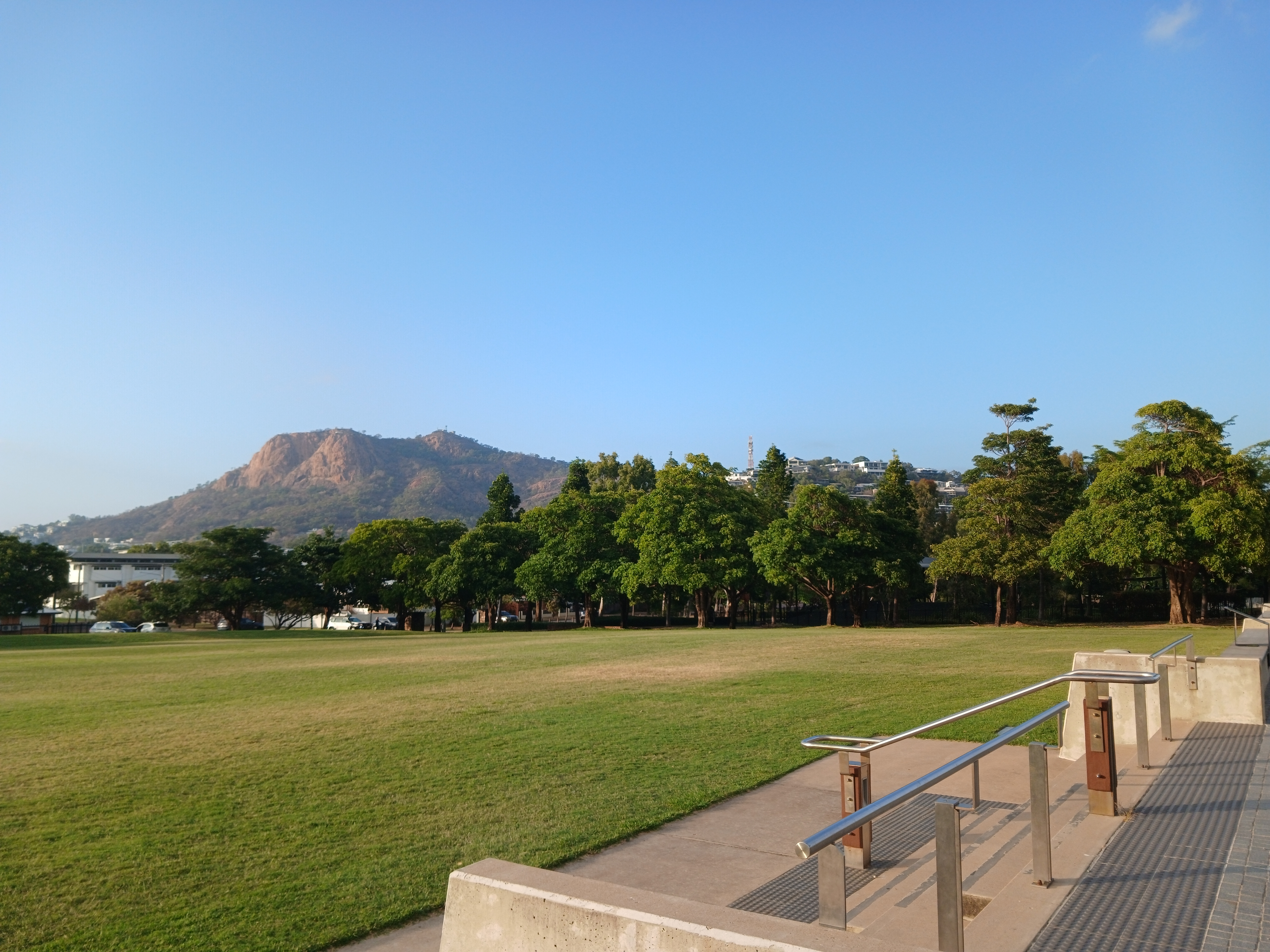
View of Castle Hill, the principal hill modelled in this article, from Jezzine Barracks.

No rolling resistance and air resistance losses

In the event of there being no non-conservative forces like rolling resistance and air resistance acting on the trike, the total energy of the system is given by:

E=T+V\begin{aligned} E &= T + V \end{aligned}

Where TT is kinetic energy (in joules) and VV is potential energy (also in joules). In turn, they are defined as:

T=mv22\begin{aligned} T=\dfrac{mv^2}{2} \end{aligned}

and

V=mgh(s).\begin{aligned} V=mgh(s). \end{aligned}

Where vv is velocity, mm is the mass of the tricycle (in kilograms), gg is gravitational acceleration (in metres per second squared (m⋅s−2\mathrm{m}\cdot \mathrm{s}^{-2})) and h(s)h(s) is the height (in mm) of the base of the tricycle above sea level. The mghmgh value for VV assumes constant gravitational acceleration.

Alternatively, if gravity is not constant:

V=GMmrbase−GMmrsummit=GMm(rbase−1−rsummit−1).\begin{aligned} V &= \dfrac{GMm}{r_{\mathrm{base}}} - \dfrac{GMm}{r_{\mathrm{summit}}}\\ &=GMm\left(r_{\mathrm{base}}^{-1}-r_{\mathrm{summit}}^{-1}\right). \end{aligned}

Where GG is the gravitational constant, MM is the mass of the Earth and rsummitr_{\mathrm{summit}} and rbaser_{\mathrm{base}} are the distances of the summit and base of the hill/mountain from the centre of the Earth.

If we are at the top of the hill and the tricycle is stationary, then E=VE=V. So, when the trike moves downhill, TT will eventually equal VV at the bottom of the hill or mountain. Hence to determine the maximum of vv we merely need to solve:

mv22=mgh.\begin{aligned} \dfrac{mv^2}{2} &= mgh. \end{aligned}

Multiplying both sides by 2m\dfrac{2}{m} yields:

v2=2gh.\begin{aligned} v^2 &= 2gh. \end{aligned}

Whereas square rooting both sides yields:

v=2gh.\begin{aligned} v &= \sqrt{2gh}. \end{aligned}

We deliberately ignored the negative solution for vv as we have defined ss to be increasing as we go downhill and hence velocity is positive in this direction. This also means that so long as motion is in the direction of downhill, which it always will be when it is moving solely under the force of gravity, velocity will always be positive.

Or, if gravity cannot be assumed constant:

mv22=GMm(rbase−1−rsummit−1)v2=2GM(rbase−1−rsummit−1).\begin{aligned} \dfrac{mv^2}{2} &= GMm\left(r_{\mathrm{base}}^{-1}-r_{\mathrm{summit}}^{-1}\right) \\ v^2 &= 2GM \left(r_{\mathrm{base}}^{-1}-r_{\mathrm{summit}}^{-1}\right). \end{aligned}

Square rooting both sides yields:

v=2GM(rbase−1−rsummit−1).\begin{aligned} v &= \sqrt{2GM\left(r_{\mathrm{base}}^{-1}-r_{\mathrm{summit}}^{-1}\right)}. \end{aligned}

Keeping in mind that the tallest point of Castle Hill is not reachable by road, so maximum altitude would be approximately somewhere in the vicinity of 265.9 metres above sea level — at least based on what Google Fit says of my altitude when I journey there. According to Equations (3) and (4), the maximum velocity of a trike travelling down Castle Hill would be approximately 260 kilometres per hour (kph).

With rolling resistance and air resistance

More realistically, however, we would expect there to be non-conservative forces acting on the trike, such as rolling resistance and aerodynamic drag. When these forces act upon the trike a simple analytical solution becomes less easy to obtain, at least if the angle of descent is allowed to not remain constant. To parametize the problem we will use an independent variable ss that will be distance, in metres, from the summit of the hill or mountain. We will assume this mountain has a road that we are travelling down and ss is the distance from the summit along this road.

Constant gravity

We will first assume that the variation in gravitational acceleration between the base and summit of the hill or mountain is negligible and derive the equation of motion based on this assumption.

Formulating the Lagrangian

The first step in deriving the equation of motion is to determine the Lagrangian of the system. The Lagrangian contains both the kinetic and potential energy of the system and hence both will be calculated next.

Kinetic energy

Substituting:

v=s˙\begin{aligned} v=\dot{s} \end{aligned}

where s˙=dsdt\dot{s}=\dfrac{ds}{dt} is the trike's velocity in m⋅s−1\mathrm{m}\cdot \mathrm{s}^{-1} into Equation (1) yields:

T=ms˙22.\begin{aligned} T=\dfrac{m\dot{s}^2}{2}. \end{aligned}

Potential energy

The potential energy term will only include the conservative force of gravitation. To compute it, we need to be able to formulate the height of the trike above sea level in terms of ss. If we have inclination/declination angle data for the hill in question, let us define θ(s)\theta(s) as the declination angle (positive when downhill) at ss metres from the summit. If we form an infinitesimal triangle on the hill/mountain, we will see that dh=−dssin⁡θdh = -d s \sin{\theta} and hence:

dhds=−sin⁡θ(s).\begin{aligned} \dfrac{dh}{ds} &= -\sin{\theta(s)}. \end{aligned}

Integrating from the summit, we obtain that:

h(s)=hsummit−∫0ssin⁡θ(σ)dσ.\begin{aligned} h(s) &= h_{\mathrm{summit}} - \int_{0}^s \sin{\theta(\sigma)}d\sigma. \end{aligned}

Where hsummith_{\mathrm{summit}} is the height of the hill/mountain, or rather its tallest point accessible by road, and we use σ\sigma as a dummy (integration) variable for distance from the summit.

Hence if gravitational acceleration can be assumed to be constant:

V=mg(hsummit−∫0ssin⁡θ(σ)dσ).\begin{aligned} V &= mg\left(h_{\mathrm{summit}} - \int_0^s \sin{\theta(\sigma)}d\sigma\right). \end{aligned}

Final Lagrangian

The Lagrangian is, by definition:

L=T−V.\begin{aligned} L &= T - V. \end{aligned}

Substituting Equations (1) and (9) into Equation (10). Therefore our Lagrangian is:

L=ms˙22−mg(hsummit−∫0ssin⁡θ(σ)dσ).\begin{aligned} L &= \dfrac{m\dot{s}^2}{2} - mg\left(h_{\mathrm{summit}} - \int_0^s \sin{\theta(\sigma)}d\sigma\right). \end{aligned}

Non-conservative forces

It is important to note, however, that nonconservative forces — such as air resistance and rolling resistance — are a major factor in determining the speed of a tricycle going downhill. To account for these effects, we need to calculate generalized forces. Fortunately, since our problem only has a single independent variable — that of distance from the summit — calculating the generalized forces should be straightforward.

Rolling resistance is proportional to the normal force. The normal force could be calculated as:

N=mgcos⁡θ(s).\begin{aligned} N=mg\cos{\theta(s)}. \end{aligned}

The rolling resistance force is defined as:

Fr=CrrN.\begin{aligned} F_r &= C_{rr}N. \end{aligned}

Where CrrC_{rr} is the coefficient of rolling resistance. Substituting Equation (12) into Equation (12) yields:

Fr=mgCrrcos⁡θ(s).\begin{aligned} F_r &= mgC_{rr}\cos{\theta(s)}. \end{aligned}

This force directly opposes motion in the direction of ss.

As for air resistance (or drag):

FD=ρCDAv22.\begin{aligned} F_D &= \dfrac{\rho C_D A v^2}{2}. \end{aligned}

Substituting Equation (5) into Equation (14) yields:

FD=ρCDAs˙22.\begin{aligned} F_D &= \dfrac{\rho C_D A \dot{s}^2}{2}. \end{aligned}

Where ρ\rho is air density in kg⋅m−3\mathrm{kg} \cdot \mathrm{m}^{-3}, CDC_D is a dimensionless drag coefficient, AA is the cross sectional surface area (in m2m^2) that the area acts on. This is also in the opposite direction to motion. Hence the generalized non-conservative forces acting on our tricycle would be:

Qs=−mgCrrcos⁡θ(s)−ρCDAs˙22.\begin{aligned} Q_s &= -mgC_{rr} \cos{\theta(s)} - \dfrac{\rho C_D A\dot{s}^2}{2}. \end{aligned}

Euler-Lagrange equation with non-conservative forces

The Euler-Lagrange equation with dissipative forces in the ss coordinate is:

ddt∂L∂s˙−∂L∂s=Qs.\begin{aligned} \dfrac{d}{dt}\dfrac{\partial L}{\partial \dot{s}} - \dfrac{\partial L}{\partial s} &= Q_s. \end{aligned}

First we shall calculate ∂L∂s˙\dfrac{\partial L}{\partial \dot{s}}, the canonical momentum:

∂L∂s˙=ms˙.\begin{aligned} \dfrac{\partial L}{\partial \dot{s}} &= m\dot{s}. \end{aligned}

Hence:

ddt∂L∂s˙=ms¨.\begin{aligned} \dfrac{d}{dt}\dfrac{\partial L}{\partial \dot{s}} &= m\ddot{s}. \end{aligned}

As for the second term in Equation (16), it is:

∂L∂s=mgsin⁡θ(s).\begin{aligned} \dfrac{\partial L}{\partial s} &= mg\sin{\theta(s)}. \end{aligned}

Hence Equation (16) becomes:

ms¨−mgsin⁡θ(s)=−mgCrrcos⁡θ(s)−ρCDAs˙22.\begin{aligned} m\ddot{s} - mg\sin{\theta(s)} &= -mgC_{rr} \cos{\theta(s)} - \dfrac{\rho C_D A\dot{s}^2}{2}. \end{aligned}

Rearranging and factorizing yields:

ms¨=mg(sin⁡θ(s)+Crrcos⁡θ(s))−ρCDAs˙22.\begin{aligned} m\ddot{s} &= mg(\sin{\theta(s)}+C_{rr}\cos{\theta(s)})-\dfrac{\rho C_D A\dot{s}^2}{2}. \end{aligned}

Dividing both sides by mm yields:

s¨=g(sin⁡θ(s)+Crrcos⁡θ(s))−ρCDAs˙22m\begin{aligned} \ddot{s} &= g(\sin{\theta(s)}+C_{rr}\cos{\theta(s)})-\dfrac{\rho C_D A\dot{s}^2}{2m} \end{aligned}

assuming constant gravitational acceleration.

Simplification to first order

s¨=ds˙dsdsdt=dsdtds˙ds=s˙ds˙ds.\begin{aligned} \ddot{s} &= \dfrac{d\dot{s}}{ds} \dfrac{ds}{dt} \\ &= \dfrac{ds}{dt} \dfrac{d\dot{s}}{ds} \\ &= \dot{s} \dfrac{d\dot{s}}{ds}. \end{aligned}

Hence Equation (18) becomes, after dividing by mm:

s˙ds˙ds=g(sin⁡θ(s)−Crrcos⁡θ(s))−ρCDAs˙22m.\begin{aligned} \dot{s} \dfrac{d\dot{s}}{ds} &= g(\sin{\theta(s)} - C_{rr} \cos{\theta(s)}) - \dfrac{\rho C_D A\dot{s}^2}{2m}. \end{aligned}

Let u=s˙2u=\dot{s}^2, then:

duds=d(s˙2)ds\begin{aligned} \dfrac{du}{ds} &= \dfrac{d(\dot{s}^2)}{ds} \end{aligned}

Hence by the chain rule:

duds=2s˙ds˙ds.\begin{aligned} \dfrac{du}{ds} &= 2\dot{s}\dfrac{d\dot{s}}{ds}. \end{aligned}

Consequently:

12duds=g(sin⁡θ(s)−Crrcos⁡θ(s))−ρCDAu2m.\begin{aligned} \dfrac{1}{2}\dfrac{du}{ds} &= g(\sin{\theta(s)} - C_{rr} \cos{\theta(s)}) - \dfrac{\rho C_D A u}{2m}. \end{aligned}

Multiplying both sides by 2 yields:

duds=2g(sin⁡θ(s)−Crrcos⁡θ(s))−ρCDAum.\begin{aligned} \dfrac{du}{ds} &= 2g(\sin{\theta(s)} - C_{rr} \cos{\theta(s)}) - \dfrac{\rho C_D A u}{m}. \end{aligned}

Solution

u(s)=C1e−CDAsm+2ge−CDAsm∫0seCDAσm(sin⁡θ(σ)−Crrcos⁡θ(σ))dσ.\begin{aligned} u(s) = C_1 e^{-\frac{C_D As}{m}} + 2ge^{-\frac{C_D As}{m}}\int_0^s e^{\frac{C_D A\sigma}{m}}(\sin{\theta(\sigma)}-C_{rr} \cos{\theta(\sigma)})d \sigma. \end{aligned}

The trike starts at the summit with zero velocity, consequently u(0)=0u(0)=0 and hence C1=0C_1=0. This simplifies u(s)u(s) to:

u(s)=2ge−CDAsm∫0seCDAσm(sin⁡θ(σ)−Crrcos⁡θ(σ))dσ.\begin{aligned} u(s) = 2ge^{-\frac{C_D As}{m}}\int_0^s e^{\frac{C_D A\sigma}{m}}(\sin{\theta(\sigma)}-C_{rr} \cos{\theta(\sigma)})d \sigma. \end{aligned}

Square rooting we obtain the velocity:

v(s)=2ge−CDAsm∫0seCDAσm(sin⁡θ(σ)−Crrcos⁡θ(σ))dσ.\begin{aligned} v(s) &= \sqrt{2ge^{-\frac{C_D As}{m}}\int_0^s e^{\frac{C_D A\sigma}{m}}(\sin{\theta(\sigma)}-C_{rr} \cos{\theta(\sigma)})d \sigma}. \end{aligned}

We neglected the negative possibility because velocity is positive in the downhill direction, which is the only direction the trike will go when under the action of gravity.

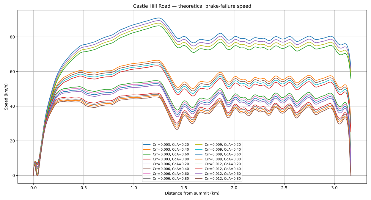
Below are the velocities achieved in the above model for various CDAC_D A and CrrC_{rr} values when descending Castle Hill. The simulation did not end at 0 metres above sea level; it ended at about 36 metres above sea level, which is approximately at the high end of Gregory Street. θ(s)\theta(s) values were calculated from QldDem data on elevation.

Velocity while descending Castle Hill, assuming constant gravity.

Non-constant gravity

Gravitational acceleration depends on the distance from the centre of the source of gravity, so there is some variation in gravitational acceleration between the base and summit of hills and mountains although it is minor. In this section, the equation of motion will be derived while accounting for this variability.

Formulating the Lagrangian

The kinetic energy we use when studying non-constant gravity is the same as before. Consequently, Equation (17) is also true for this Lagrangian.

Potential energy

If we cannot assume constant gravity, then:

V=GMm(rbase+h(s))−GMmrsummit.\begin{aligned} V &=\dfrac{GMm}{(r_{\mathrm{base}} + h(s))} - \dfrac{GMm}{r_{\mathrm{summit}}}. \end{aligned}

Factorizing:

V=GMm((rbase+h(s))−1−rsummit−1).\begin{aligned} V &= GMm\left((r_{\mathrm{base}} + h(s))^{-1} - r_{\mathrm{summit}}^{-1}\right). \end{aligned}

Where GG is the gravitational constant and MM is the mass of the Earth.

Substituting Equation (8) into Equation (23) yields:

V=GMm[(rsummit−∫0ssin⁡θ(σ)dσ)−1−rsummit−1].\begin{aligned} V &= GMm\left[\left(r_{\mathrm{summit}} - \int_0^s \sin{\theta(\sigma)}d\sigma\right)^{-1}-r_{\mathrm{summit}}^{-1}\right]. \end{aligned}

Final Lagrangian

Or, if gravitational acceleration cannot be assumed to be constant:

L=ms˙22−GMm[(rsummit−∫0ssin⁡θ(σ)dσ)−1−rsummit−1].\begin{aligned} L &= \dfrac{m\dot{s}^2}{2} - GMm\left[\left(r_{\mathrm{summit}} - \int_0^s \sin{\theta(\sigma)}d\sigma\right)^{-1}-r_{\mathrm{summit}}^{-1}\right]. \end{aligned}

Non-conservative forces

If gravity cannot be assumed to be constant then:

g=GM(rsummit−∫0ssin⁡θ(σ)dσ)2.\begin{aligned} g=\dfrac{GM}{\left(r_{\mathrm{summit}} - \int_0^s \sin{\theta(\sigma)}d\sigma\right)^2}. \end{aligned}

Substituting Equation (23) into Equation (13) yields:

Fr=GMmCrrcos⁡θ(s)(rsummit−∫0ssin⁡θ(σ)dσ)2\begin{aligned} F_r &= \dfrac{GMmC_{rr}\cos{\theta(s)}}{\left(r_{\mathrm{summit}} - \int_0^s \sin{\theta(\sigma)}d\sigma\right)^2} \end{aligned}

Computing Equation (16)

The conservative force term of the Euler-Lagrange equation is therefore:

∂L∂s=GMmsin⁡θ(s)(rsummit−∫0ssin⁡θ(σ)dσ)2.\begin{aligned} \dfrac{\partial L}{\partial s} &= \dfrac{GMm\sin{\theta(s)}}{\left(r_{\mathrm{summit}} - \int_0^s \sin{\theta(\sigma)}d\sigma\right)^2}. \end{aligned}

The time derivative of generalized momentum is the same as above. As for QsQ_s it is:

Qs=−GMmCrrcos⁡θ(s)(rsummit−∫0ssin⁡θ(σ)dσ)2−ρCDAs˙22.\begin{aligned} Q_s &= -\dfrac{GMmC_{rr}\cos{\theta(s)}}{\left(r_{\mathrm{summit}} - \int_0^s \sin{\theta(\sigma)}d\sigma\right)^2} - \dfrac{\rho C_D A \dot{s}^2}{2}. \end{aligned}

Substituting Equations (25) and (26) into Equation (16) yields:

ms¨−GMmsin⁡θ(s)(rsummit−∫0ssin⁡θ(σ)dσ)2=−GMmCrrcos⁡θ(s)(rsummit−∫0ssin⁡θ(σ)dσ)2−ρCDAs˙22.\begin{aligned} m\ddot{s} - \dfrac{GMm\sin{\theta(s)}}{\left(r_{\mathrm{summit}} - \int_0^s \sin{\theta(\sigma)}d\sigma\right)^2} &= -\dfrac{GMmC_{rr}\cos{\theta(s)}}{\left(r_{\mathrm{summit}} - \int_0^s \sin{\theta(\sigma)}d\sigma\right)^2} - \dfrac{\rho C_D A\dot{s}^2}{2}. \end{aligned}

Rearranging and factorizing:

ms¨=GMm(rsummit−∫0ssin⁡θ(σ)dσ)2[sin⁡θ(s)−Crrcos⁡θ(s)]−ρCDAs˙22s¨=GM(rsummit−∫0ssin⁡θ(σ)dσ)2[sin⁡θ(s)−Crrcos⁡θ(s)]−ρCDAs˙22m.\begin{aligned} m\ddot{s} &= \dfrac{GMm}{\left(r_{\mathrm{summit}} - \int_0^s \sin{\theta(\sigma)}d\sigma\right)^2} \left[\sin{\theta(s)}-C_{rr}\cos{\theta(s)}\right] - \dfrac{\rho C_D A\dot{s}^2}{2} \\ \ddot{s} &= \dfrac{GM}{\left(r_{\mathrm{summit}} - \int_0^s \sin{\theta(\sigma)}d\sigma\right)^2} \left[\sin{\theta(s)}-C_{rr}\cos{\theta(s)}\right] - \dfrac{\rho C_D A\dot{s}^2}{2m}. \end{aligned}

Simplification to first order

s¨=s˙ds˙ds\ddot{s} = \dot{s} \dfrac{d\dot{s}}{ds} hence Equation (27) becomes:

s˙ds˙ds=GM(rsummit−∫0ssin⁡θ(σ)dσ)2[sin⁡θ(s)−Crrcos⁡θ(s)]−ρCDAs˙22m.\begin{aligned} \dot{s} \dfrac{d\dot{s}}{ds} &= \dfrac{GM}{\left(r_{\mathrm{summit}} - \int_0^s \sin{\theta(\sigma)}d\sigma\right)^2} \left[\sin{\theta(s)}-C_{rr}\cos{\theta(s)}\right] - \dfrac{\rho C_D A\dot{s}^2}{2m}. \end{aligned}

Letting u=s˙2u=\dot{s}^2, then duds=2s˙ds˙ds\dfrac{du}{ds} = 2\dot{s}\dfrac{d\dot{s}}{ds} and so:

12duds=GM(rsummit−∫0ssin⁡θ(σ)dσ)2[sin⁡θ(s)−Crrcos⁡θ(s)]−ρCDAu2m.\begin{aligned} \dfrac{1}{2}\dfrac{du}{ds} &= \dfrac{GM}{\left(r_{\mathrm{summit}} - \int_0^s \sin{\theta(\sigma)}d\sigma\right)^2} \left[\sin{\theta(s)}-C_{rr}\cos{\theta(s)}\right] - \dfrac{\rho C_D A u}{2m}. \end{aligned}

Multiplying both sides by 2 yields:

duds=2GM(rsummit−∫0ssin⁡θ(σ)dσ)2[sin⁡θ(s)−Crrcos⁡θ(s)]−ρCDAum.\begin{aligned} \dfrac{du}{ds} &= \dfrac{2GM}{\left(r_{\mathrm{summit}} - \int_0^s \sin{\theta(\sigma)}d\sigma\right)^2} \left[\sin{\theta(s)}-C_{rr}\cos{\theta(s)}\right] - \dfrac{\rho C_D A u}{m}. \end{aligned}

Solution

Hence:

u(s)=C1e−CDAsm+2GMe−CDAsm∫0seCDAσmsin⁡θ(σ)−Crrcos⁡θ(σ)(rsummit−∫0σsin⁡θ(ξ)dξ)2dσ.\begin{aligned} u(s) = C_1 e^{-\frac{C_D As}{m}} + 2GMe^{-\frac{C_D As}{m}}\int_0^s e^{\frac{C_D A\sigma}{m}}\dfrac{\sin{\theta(\sigma)}-C_{rr} \cos{\theta(\sigma)}}{\left(r_{\mathrm{summit}}-\int_0^\sigma \sin{\theta(\xi)} d\xi\right)^2} d \sigma. \end{aligned}

Yet again u(0)=0u(0)=0 means C1=0C_1=0 and hence:

u(s)=2GMe−CDAsm∫0seCDAσmsin⁡θ(σ)−Crrcos⁡θ(σ)(rsummit−∫0σsin⁡θ(ξ)dξ)2dσ.\begin{aligned} u(s) &= 2GMe^{-\frac{C_D As}{m}}\int_0^s e^{\frac{C_D A\sigma}{m}}\dfrac{\sin{\theta(\sigma)}-C_{rr} \cos{\theta(\sigma)}}{\left(r_{\mathrm{summit}}-\int_0^\sigma \sin{\theta(\xi)} d\xi\right)^2} d \sigma. \end{aligned}

Square rooting uu to obtain velocity yields:

v(s)=2GMe−CDAsm∫0seCDAσmsin⁡θ(σ)−Crrcos⁡θ(σ)(rsummit−∫0σsin⁡θ(ξ)dξ)2dσ.\begin{aligned} v(s) &= \sqrt{2GMe^{-\frac{C_D As}{m}}\int_0^s e^{\frac{C_D A\sigma}{m}}\dfrac{\sin{\theta(\sigma)}-C_{rr} \cos{\theta(\sigma)}}{\left(r_{\mathrm{summit}}-\int_0^\sigma \sin{\theta(\xi)} d\xi\right)^2} d \sigma}. \end{aligned}

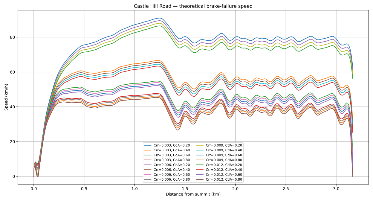
Below are the velocities achieved in the above model for various CDAC_D A and CrrC_{rr} values when descending Castle Hill. The simulation did not end at 0 metres above sea level; it ended at about 36 metres above sea level, which is approximately at the high end of Gregory Street.

Velocity while descending Castle Hill, assuming non-constant gravity.