FunctionIntegrator.jl should be treated as a second-rate alternative to the excellent QuadGK package. QuadGK provides more accurate integration for many problems, and also provides an error estimate which functions in this package do not.
use Julia's help function (e.g. by typing ?chebyshev_quadrature) to find out usage information, should you need it. The choice of function table below also explains some of the details of each of these functions, such as their arguments.
This package is currently in Julia's General registry, thus to install it one merely needs to run:
As a general rule of thumb, adaptive_simpsons_rule should be the function you use when you are unsure which function to use, as its accuracy is more predictable. The main time when adaptive_simpsons_rule should be avoided is when there are unremovable singularities at the endpoints of the domain of integration, in which case using chebyshev_quadrature with k=1 or using legendre_quadrature is likely best.
Each of the functions whose name ends with _quadrature uses Gaussian quadrature, the specifics of which differ between functions. Out of them, legendre_quadrature is perhaps the best to go with when you are uncertain which out of the _quadrature functions to go with as it can be applied to any grid and any problem and usually arrives at a result that is accurate to at least seven significant figures provided N≥1×10⁴. legendre_quadrature has the added benefit of being perhaps the fastest _quadrature function after controlling for accuracy of the result obtained.
The test/ folder has test scripts that approximate various different integrals (each file, except test/runtests.jl, pertains to a different integral); the N values given are the smallest possible to pass each of the tests listed (except when the test involves a less than (<) sign). If you want to know which function to use for which integral is these tests may be useful as a rough guide.
Figure 1: a bar graph to compare the computation times for each fo the flexible-domain methods provided by the package except for rectange_rule_left and rectangle_rule_right.1 Data is from this build.
Function
Domain2
Weight
Arguments
Notes
adaptive_simpsons_rule
[a,b]
N/A
f is the function being integrated. ε is the relative tolerance in the solution (that is, the maximum amount of relative error in the solution you are willing to tolerate). a is the start of the domain of integration. b is the end of the domain of integration.
f is the function being integrated. N is the number of grid points. k is the type of Chebyshev quadrature being used. 1, 2, 3, and 4 refer to the Chebyshev Tn, Un, Vn and Wn polynomials respectively. a is the start of the domain of integration. b is the end of the domain of integration.
Uses Chebyshev-Gauss quadrature (note this article does not mention 3rd and 4th quadrature types, corresponding to k=3 and k=4, respectively). If there are unremovable singularities at the endpoints, it with k=1 or legendre_quadrature are preferred.
hermite_quadrature
[−∞,∞]
e−x2
f is the function being integrated. N is the number of grid points. k determines the problem being solved (whether e−x2 is assumed to be part of the integrand (k=2) or not).
Uses Gauss-Hermite quadrature. Only use this if your integration domain is [−∞,∞] and your integrand rapidly goes to zero as the absolute value of x gets larger.
jacobi_quadrature
[a,b] −1≤x≤1
(1−x)α(1+x)β
f is the function being integrated. N is the number of grid points. α and β are parameters of the weighting function. a is the start of the domain of integration. b is the end of the domain of integration.
Uses Gauss-Jacobi quadrature. After controlling for N it is one of the slowest quadrature methods. A condition of Gauss-Jacobi quadrature is that α,β>−1. When α=β=0, this reduces to legendre_quadrature.
laguerre_quadrature
[0,∞]
e−x
f is the function being integrated. N is the number of grid points. k determines the problem being solved (whether e−x is assumed to be part of the integrand (k=2) or not).
Uses Gauss-Laguerre quadrature. Only use this if your integration domain is [0,∞] and your integrand rapidly goes to 0 as x gets larger.
legendre_quadrature
[a,b] −1≤x≤1
1
f is the function being integrated. N is the number of grid points. a is the start of the domain of integration. b is the end of the domain of integration.
Uses Gauss-Legendre quadrature. Generally, this is the best _quadrature function to go with when you are otherwise unsure which to go with.
lobatto_quadrature
[a,b] −1≤x≤1
1
f is the function being integrated. N is the number of grid points. a is the start of the domain of integration. b is the end of the domain of integration.
Uses Gauss-Lobatto quadrature. This function includes, in the calculation is the values of the integrand at one of the endpoints. Consequently, if there are unremovable singularities at the endpoints, this function may fail to give an accurate result even if you adjust the endpoints slightly to avoid the singularities.
radau_quadrature
[a,b] −1≤x≤1
1
f is the function being integrated. N is the number of grid points. a is the start of the domain of integration. b is the end of the domain of integration.
Uses Gauss–Radau quadrature, for which there is no Wikipedia article is the best article (simplest) I could find on it are these lecture notes. This function includes, in the calculation is the values of the function at the endpoints. Consequently, if there are unremovable singularities at either or both of the endpoints, this function will fail to give an accurate result even if you adjust the endpoints slightly to avoid the singularities.
rectangle_rule_left
[a,b]
N/A
f is the function being integrated. N. N is the number of grid points used in the integration. a is the start of the domain of integration. b is the end of the domain of integration.
Uses the rectangle rule, specifically the left Riemann sum. Usually this or rectangle_rule_right is the least accurate method. In fact, many of the tests in the FunctionIntegrator.jl repository fail to get accuracy to 7 significant figures with rectangle_rule_left with any practically viable value of N.
rectangle_rule_midpoint
[a,b]
N/A
f is the function being integrated. N. N is the number of grid points used in the integration. a is the start of the domain of integration. b is the end of the domain of integration.
Uses the rectangle rule, specifically the Riemann midpoint rule. Usually this is more accurate than rectangle_rule_left and rectangle_rule_right and sometimes rivals trapezoidal_rule for accuracy. Interestingly, going by my Travis tests it appears to be even more efficient than simpsons_rule.
rectangle_rule_right
[a,b]
N/A
f is the function being integrated. N. N is the number of grid points used in the integration. a is the start of the domain of integration. b is the end of the domain of integration.
Uses the rectangle rule, specifically the right Riemann sum. Usually this or rectangle_rule_left is the least accurate method. In fact, many of the tests in the FunctionIntegrator.jl repository fail to get accuracy to 7 significant figures with rectangle_rule_right with any practically viable value of N.
rombergs_method
[a,b]
N/A
f is the function being integrated. N. Equal to n in this article that describes the method. a is the start of the domain of integration. b is the end of the domain of integration.
Uses Romberg's method. If your PC has only 16 GB RAM, you should not exceed N=30, as otherwise you will likely run out of RAM. For most problems, N≤20 should suffice.
simpsons_rule
[a,b]
N/A
f is the function being integrated. N. N+1 is the number of grid points, if endpoints are included. N must be even, otherwise this function will throw an error. a is the start of the domain of integration. b is the end of the domain of integration.
Uses Simpson's rule. It is one of the best functions to use when you are unsure which to use, provided there are no unremovable singularities within the integration domain, including the endpoints.
simpsons38_rule
[a,b]
N/A
f is the function being integrated. N. N+1 is the number of grid points, if endpoints are included. N must be divisible by three, as otherwise this function will throw an error. a is the start of the domain of integration. b is the end of the domain of integration.
f is the function being integrated. N. N+1 is the number of grid points, if endpoints are included. a is the start of the domain of integration. b is the end of the domain of integration.
Uses the trapezoidal rule. It has the same caveats as simpsons_rule.
Notes:
rectangle_rule_left, rectangle_rule_midpoint and rectangle_rule_right are not included because they failed to provide the required level of accuracy for many tests with all practically viable N values.
The −1≤x≤1 refers to the quadrature nodes, which are also referred to in the weighting function column.
In the following examples, integral 1 is being computing and the result compared to the analytical solution of 1. The value being printed is difference between the computed solution and the analytical solution.
k=1:
using FunctionIntegrator
a = abs(chebyshev_quadrature(x -> cos(x), 1000, 1, 0, pi/2) - 1);
show(a)
3.229819232064557e-7
k=2:
using FunctionIntegrator
a = abs(chebyshev_quadrature(x -> cos(x), 1000, 2, 0, pi/2) - 1);
show(a)
6.446739609922147e-7
k=3:
using FunctionIntegrator
a = abs(chebyshev_quadrature(x -> cos(x), 1000, 3, 0, pi/2) - 1);
show(a)
6.453189426158801e-7
k=4:
using FunctionIntegrator
a = abs(chebyshev_quadrature(x -> cos(x), 1000, 4, 0, pi/2) - 1);
show(a)
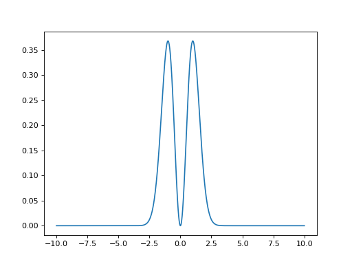
the exact solution of which is 2π, will be approximated using hermite_quadrature and the result will be compared to the analytical solution. The plot of the integrand is (truncated to the domain x∈[−10,10]):
using PyPlot
x = LinRange(-10,10,1001);
clf()
y = (x.^2).*exp.(-x.^2);
PyPlot.plot(x,y)
PyPlot.savefig(joinpath(@OUTPUT, "hermite_plot.png"), dpi=80)
k=1:
using FunctionIntegrator
a = abs(hermite_quadrature(x -> x^2*exp(-x^2), 100, 1)-sqrt(pi)/2)
show(a)
2.6645352591003757e-15
k=2:
using FunctionIntegrator
a = abs(hermite_quadrature(x -> x^2, 100, 2)-sqrt(pi)/2)
show(a)
In this example, we will approximate integral 1 and compare the result to the analytical result of 1. For this example, we are setting both α and β to 1.
using FunctionIntegrator
a = abs(jacobi_quadrature(x -> cos(x), 1000, 1, 1, 0, pi/2)-1);
show(a)
MethodError: no method matching asy1(::Int64, ::Int64, ::Int64, ::Int64)
The function `asy1` exists, but no method is defined for this combination of argument types.

Closest candidates are:
  asy1(::Integer, !Matched::Float64, !Matched::Float64, ::Integer)
   @ FastGaussQuadrature ~/.julia/packages/FastGaussQuadrature/BRLTf/src/gaussjacobi.jl:200
I would like to thank the Julia discourse community for their help through my Julia journey, and I would also like to thank the developers of Julia, as without their work this package would not even be possible (I know, obviously, as this is a Julia package). Likewise, I would also like to thank the developers of FastGaussQuadrature.jl, as without their efficient algorithms for finding the nodes and weights for various Gaussian quadrature techniques, several of the functions in this repository would be far less efficient (especially legendre_quadrature), or may not even exist. I would also like to thank the developers of SpecialFunctions.jl, as some of their functions are useful for testing the functions in this package.